Face Detection based on Boosting Machine

Boosting is a general method to improve the performance on classification or regression tasks by combining weak learners, even when they are only slightly better than random guess to form an arbitrarily good hypothesis. Face detection is in essense a binary classification problem of patches extracted from a image.

In this project, we train on over 11838 faces and 25356 non-faces examples, to select from 10032 weak classifiers and ensemble them to a strong classifier for face detection on a classroom photo. We invetigate adaboost and realboost for the classifcation, and also intruduce techniques including Haar image filter, hard-negtive mining and non-maximum suppression

1. Weak Classifier - Haar Filters

Haar filter operates in a detection window by divding the patch into rectangular regions and calculating the difference between pixel intensities sums in the regions. This difference is then used as the feature of this subsections of an image. The key advantage of it is the computation efficiency. Using integral images, a Haar-like feature of any size can be calculated in constant time.

In this experiment we build weak classifiers for human face based on haar filters. Each filter is a type of filter applied on a specific detection window, hence each image $x$ is associated with a value with respect to each filter. Thus, a weak classifier $h_t(x)$ is then defined by a threshold $\theta_j$ that optimally seperates positive and negative examples. $$h_t(x) = 1 \quad if \quad haar_t(x)>\theta_t \quad else \quad -1$$

In order to choose the optimal threshold $\theta_t$, we first equally divide the range of all values into a number of candicate thresholds (25 in our experiments), and choose the threshold and the polarity ($s_t \in \{-1, 1\}$) with the lowest error rate.

$$h_t(x) = s_t \quad if \quad haar_t(x)>\theta_j \quad else \quad -s_t$$

In Figure 1 we display the top 20 haar filters after adaboost training. Here we rank the filters by the classifier weights $\alpha_t$ which indicates the importance of the weak classifer in the final decision.

Fig.1

2. Adaboost - Weighted Binary Votes

Adaboost is a linear combination of weak classifiers, and can be analogous to a commettee decision process. It makes finding the linear weight $\alpha_t$ for each classifier the primary challenge. The intuition behind adaboost (adaptive boosting) is to iteratively update the model by choosing a current best weak classifer on the residual from the previous model, by fitting residual it means to reweight the observations by $D_i=e^{-y_1f_{t-1}(x_i)}$ such that those were wrongly classified are more emphsized with higher weights. By the deduction of exponential loss below we obtain the updates for $\alpha_t = \frac{1}{2} log \frac{1-\epsilon_{t}}{\epsilon_{t}}$.

$$\hat{y} = sign(F(x)) = sign(\sum_t f_t(x)) = sign(\sum_t \alpha_t\cdot h_t(x)) $$

$$Loss_t=\frac{1}{Z}\sum_{i=1}^n e^{-y_i f(x_i)} \propto e^{-y_i f(x_i)} =\sum_{i=1}^n e^{-(y_i f_{t-1}(x_i)+\alpha_{t}y_i h_t(x_i))} = \sum_{y_i=h_t(x_i)} e^{-y_i f_{t-1}(x_i)} e^{-\alpha_{t}} + \sum_{y_i=h_t(x_i)} e^{-y_i f_{t-1}(x_i)} e^{\alpha_{t}} \\ = \sum_{y_i=h_t(x_i)} D_i e^{-\alpha_{t}} + \sum_{y_i=h_t(x_i)} D_i e^{\alpha_{t}} = (1-\epsilon_{t})e^{-\alpha_{t}} + \epsilon_{t} e^{\alpha_{t}}$$

$$\quad \because \sum_{i}D_i = 1, \qquad argmin(Loss) \quad \rightarrow \quad \alpha_t = \frac{1}{2} log \frac{1-\epsilon_{t}}{\epsilon_{t}}$$

In our experiment, we run adaboost to find 100 weak classifiers. It can be observed from Figure 2 that training error descrease monotonely and reached an training accuracy of .94. Figure 3 diplays the training error of the first 1000 weak classifier at different time step. In each iteration, there are several weak classifiers has errors significantly smaller than the others, while this difference is diminishing as the minimum error increase, because the previous strong classifier is performing better and better.

Fig.2	Fig.3

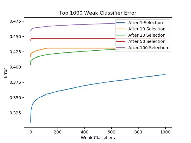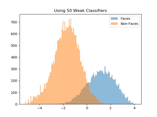
Figure 4 displays the histograms of scores with T=10, 20, 50, 100 weak classifiers. As the number of weak classifiers increase, positive examples and negtive examples are better seperated. Moreover, the scores in each class tend to distribute in a bell-shape. It can be explained by CLT that the sum of a large number of independent random variables tends toward a normal distribution.

Fig.4a 10 weak classifiers	Fig.4b 20 weak classifiers	Fig.4c 50 weak classifiers	Fig.4d 100 weak classifiers

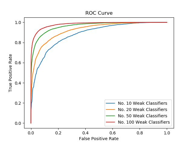
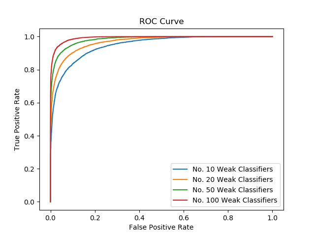
ROC curve in Figure 5 shows the false positive rate and true positive rate with different final decision threshold. The space under the curve indicates the accuracy which is in accordance with that from error rate.

Fig.5

3. Detection on real image - nonmaximum suppression

With the adboost model built with 100 weak classifiers, we detect faces from a real classroom photo. Notice that when sliding the detection window across the image, we rescale the image into 20 different scales and extract the $16 \times 16$ detection targets in order to check faces with different sizes.

Moreover, it is common that the detected regions overlaps a lot since nearby regions may have similar score. Therefore, we perform non-maximum suppression to keep only the one with the highest score if two images has overlapping area. In computation, we sort the scores in decending order and find all overlapping patches near the first patch and then move to the second etc.

The resulted detection is marked in Figure 6. Although most faces, even small and obscure ones at the back are detected, we can observe mant false positive prediction. It is understandable as there are infinite non-face examples that are not seen by the model in training stage, which is why we introduce hard negtive mining.

Fig.6a	Fig.6b

4. Hard Negative Mining

To increase the performance, we use negative examples that are faultly predicted as face in three background images as new training examples and continue training for 100 iterations.

In the experiment we obtain 15149 negative examples. With those new data, we retrain the model to o

By this way we obtain a even higher training accuracy at .97. In figure7-b we compare the significant improvement made by negative mining, the result before mining is marked in green while those after are marked in red.

Fig.7a Hard Negtive Mining Detection	Fig.7b Hard Negtive Mining compared to the previous detection

Fig.7c Hard Negtive Mining Detection	Fig.7d Hard Negtive Mining with a .7 threshold

We also try to improve the performance by increase the final decision threshold from 0 to 0.7 to reserve only half of the detected faces. It is a effective way to control false positive as suggested by Figure 7-c and d, also we may further increase the threshold to get all solid faces while some faces may not be detected. However, the choice of the threshold deserves further discussion.

3. Realboost - Vote by a real number

In adaboost, we define each classifier by partition the whole data into two parts by a threshold and assign the classifier a weight computed from the error rate of this partition. An extention is to absorb the weight $\alpha$ into the label assignment such that we can partition the data into more parts (bins) and allows for different (and more accurate in general) decisions in each bin. It is like each classifier vote on an example by a real number according to the training examples falls into the same bin with it.

We define error ($1-\epsilon$) and accracy ($\epsilon$) in each bin as:

$$p_t(b)=\sum_i D_i I[y_i=+1] I[x_i \in bin_b], \quad q_t(b)=\sum_i D_i I[y_i=-1] I[x_i \in bin_b]$$

Thus,

$$\hat{y} = sign(F(x)) = sign(\sum_t f_t(x)), \quad f_t(x) = \sum_b I[x \in bin_b] h_{t,b} $$

$$Loss_t \propto \sum_{i=1}^n exp(-y_i f(x_i)) = \sum_{i=1}^n D_i e^{-y_i h_{t,b}} = \sum_{b} D_i p_t(b) e^{-h_{t,b}} + q_t(b) e^{h_{t,b}}$$

$$argmin(Loss) \quad \rightarrow \quad h_{t,b}= \frac{1}{2} log \frac{p_t(b)}{q_t(b)}$$

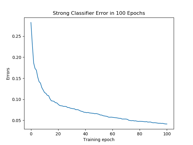
To simplify the computation, we use the 100 filters chosen by adaboost and recaculating their weights with all training examples (including negative examples), not surprisingly we achieve a better training accuracy. Whereas the reulted detection is no better than Adaboost.

Fig.8 Realboost Weighting Train Error

Fig.9a Realboosting Weights Detection	Fig.9b Adaboost detection

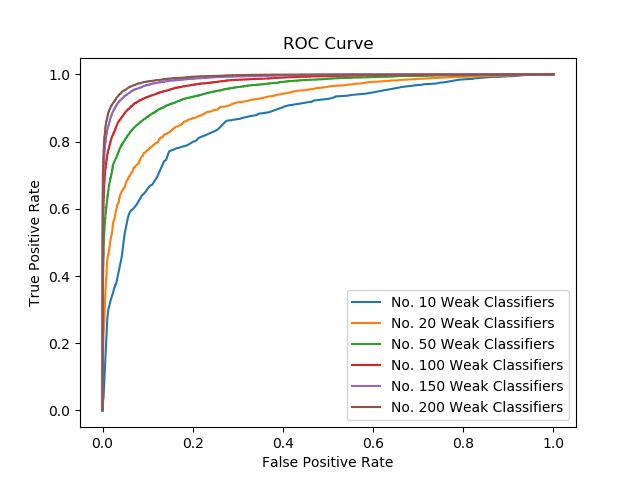
We compare the histograms and roc curve below (both with negative mined examples):

Fig.10a 10 weak classifiers	Fig.4b 50 weak classifiers	Fig.4c 100 weak classifiers	Fig.4d ROC Curve
Adaboost Case	Adaboost Case	Adaboost Case	Adaboost Case
----	----	----	----