Face Image Recognition

--- Compression & Discrimination by PCA, AutoEncoder, FLD

Jiayu WU | 905054229

This project aims to explore face recognition by extracting effective compression and representations of face images.

Firstly, we start with the classical principal component analysis for dimension reduction and generation from the latent components. In order to address different aspects of the images - face apperance and photographing angles, we decompose the two aspects by image alignment by warping according to landmarks.

In addition, we generalize linear projection of PCA onto latent space to a more flexible nonlinear projection learned by neural network, which is AutoEncoder, a effective way to compress high dimensional, sparse data.

At last, we explore Fisher Linear Discriminant, a discriminative method by linear projection that tells apart female and male faces.

We experiemnt with a dataset of 1000 face imgaes with 256 x 256 pixels, of which 588 are males and 412 females. They are pre-processed such that the background and hair are removed and the faces have similar lighting. Each face has 68 landmarks manually identified. The dataset is split into training/testing set with testing size of 200.

1. PCA - dimension reduction

1.1 PCA on Raw Image

As PCA is usually applied on the intensity, in our experiment the color image is converted to the HSV and PCA is applied on the Value channel.

Applying PCA on the 800 training examples by SVD decomposition, we obtain eigen faces sorted by 'importance' or 'amount of infomation' - the total variance explained. The First 20 faces are displayed in Fig.1-1-1.

Fig.1-1-1

Although the raw image data (V channel) is in a very high-dim space of $N^2=128 \times 128$, we show that the image can be reconstructed to high resemblence to the original using only the first 50 eigen faces, as diplayed in Fig.1-1-2 using 20 testing images. We also compare the reconstrution errors (average MSE normalized by pixel)on the 200 testing images with different numbers of eigenfaces in Fig.1-1-3.

Fig.1-1-2

The reconstructed faces are close enough to the original to be recognized, despiet the loss in clarity.

Fig.1-1-3

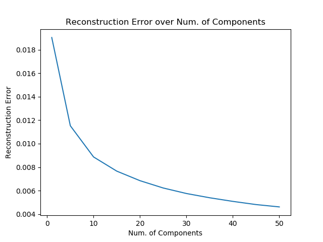It can be observed that, the err decrease more and more slowly as the number eigenfaces used in reconstruction increase, and it diminish to less than $.005$ with only 50 eigenfaces (the raw data dimenionality is 300 times higher). It can be concluded that high-dim, sparse data like image pixels can be effectively compressed to a lower space for modeling.

1.2. PCA on landmarks for warping

Since in the image the faces have different angles, it is very reasonable to align (image warping) them to a mean position before extracting appearance components. It is notable that the identified landmarks can also be reconstructed by PCA, such that we deal with a lower space than the original ($68\time 2$).

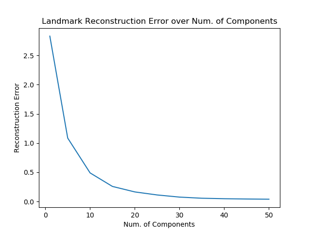
The eigen landmarks and resonstruction errors are ploted in Fig.1-2-1 and Fig.1-2-2 respectively. The error here is defined as the distance on the 2-dim plane. A sharp drop in error can be observed within the first 10 eigen lanmarks, therefore we believe 10 eigen warping will be good enough.

Fig.1-2-1

Fig.1-2-2

1.2. PCA with landmarks alignment

Combining the two steps above, we reconstruct images based on top-10 eigen landmarks for the warping and then top-50 eigen faces for the appearance.

Fig.1-3-1a	Fig.1-3-1b	Fig.1-3-1c

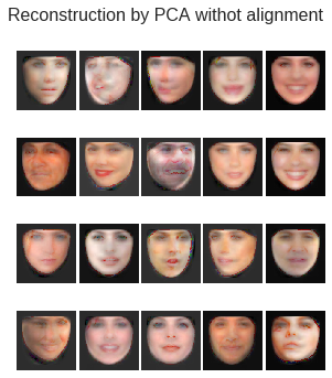The restored faces in contrast to the original testing examples are displayed in Fig.1-3-1. It shows that with alignment, the reconstruction image become more clear and more robust. Specificly, it handels significantly better the varying geometry differing from the mean position, ex. faces not facing the front, also more details, like wrinkles, can be recontructed

The reconstruction errors in Fig.1-3-2 is larger than the of image without alignment. It is plausible as here we have two aparts of loss form the geometry and from the appearance. In our experiment the geometry error is constantly at 0.49.

Fig.1-3-2

1.3. Generation by sampling

With principle componants from PCA, unseen samples of face image can be generated by sampling the weights. Assuming normal distribution for the latent componants, we have mean 0 (data centered for PCA) and the variance (eigen value). 20 sampled faces is show in Fig 1-3-3. The faces in those images are all recognizable, though some are distorted due to the variation in sampling. Moreover, a evitable drawback in this method is that PCA only handle the intensity level of the image, thus lose the color informtion in the original data.

Fig.1-3-3

2. AutoEncoder - nonlinear generalization

2.1 AutoEncoder with alignment

Extending the dimension reduction idea of PCA, AutoEncoder uses a more flexible nonlinear projection learned by neural network through minimization of reconstruction mean square error. Replacing PCA in the previous section with autoencoder, we obtain the reconstructed faces in Fig. 2-1a. Note that AutoEncoder is able to handle color image naturally using convolutional layers, rathan than operate on the in intensity level.

Fig.2-1a	Fig.2-1b	Fig.2-1c

Compared with those reconstructed from PCA, AutoEncoder is very sensitive to change of intensity with the ability to learn very detailed features. However, it tends to overfit and thus exagerate the features, even though adding .8 dropout rate for appearance model has resolved the problem to some extent as shown in Fig. 2-1d.

Fig.2-2d

2.2 Interpolation

In this section, we synthesis new images with latent dimension variations. Each time we choose 10 values equally spaced between the training mean $+/-$ 2 standard errors of one latent variable, while fixing others. Note that for appearance we use the model without dropout layer to make the features more visible, and for landmark we operate on the average appearance.

Fig.2-2a

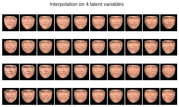In Fig.2-2a, we can observe a clear change of dictinct features on the first four latent appearance variables relected in each row: nose, eyes, eyes and mouth, while in the center there is the mean image with an average face.

Fig.2-2b	Fig.2-2c

In Fig.2-2b and c, variations in direction and shape of the face is evident.

3. FLD - discrimination by linear projection

3.1 Fisher face discrimination

Fisher Linear discrimination finds a set of shared weights that project the high dimensional data to one-dim points that separates the different classes optimally. Using the image data compressed by PCA (50-dim), we can find the fisher face that best seperates male and female faces with a $86 \%$ accuracy rate on the $200$ testing examples. It also indicates that the PCA compressed data is representative and descriptive by reserving main information from the original high-dim images.

Fig.3-1

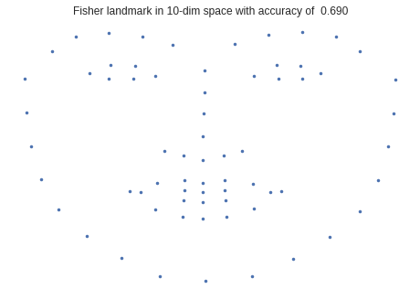
3.2 Visualization on 2D feature space

Since both appearance and geometry features can be obtained from the face images, we apply FLD on both features thus each image is projected to a 2D plane. The testing images are thus visualized in Fig.3-2a, where blue dots are male examples.

Fig.3-2a	Fig.3-2b	Fig.3-2c